Stitching Vision into LLMs: A Comparative Analysis of Embedding Spaces
Building a VLM from scratch using model stitching and LoRA — comparing CLIP's language alignment vs. I-JEPA's world modeling.
I’ve been thinking a lot about world models lately. The kind of models that don’t just classify what they see, but actually understand the structure of the visual world—objects, spatial relationships, how things fit together. If we’re ever going to build AI systems that can genuinely reason about images (or, you know, operate a computer), the vision encoder is doing all the heavy lifting up front. It’s the bottleneck. And most people just default to CLIP and move on.
That felt unsatisfying to me.
I initially wanted to experiment with V-JEPA (Video Joint-Embedding Predictive Architecture) Meta’s video-native world model. V-JEPA is fascinating because it learns by predicting missing spatiotemporal regions of video in a learned latent space, without requiring any labels or text. It’s essentially building an internal physics engine from raw video. But V-JEPA is more about action-conditioned prediction and temporal dynamics—you’re really in the territory of planning and control, not static visual understanding. The compute requirements are also non-trivial; it’s designed for video pretraining at scale with masking schedules across both space and time dimensions.
So I stepped back to I-JEPA (Image JEPA), its image-only predecessor. Same core idea—predict masked regions in latent space—but operating on single images. Much more tractable for the experiment I had in mind.
The question I wanted to answer was simple: if you freeze a vision encoder and stitch it into an LLM, does the encoder’s pre-training strategy actually matter for downstream VLM performance?
Spoiler: it does. But not always in the way you’d expect.
What Are World Models, and Why Should You Care?
A “world model” is a learned internal representation of how the environment works. Instead of just mapping inputs to outputs, a world model captures structure—spatial relationships, object permanence, cause and effect. Think of it as the difference between a model that can label “dog” and a model that understands the dog is sitting on a couch, next to a person, in front of a window.
This matters because the next generation of AI systems—robotic manipulation, autonomous agents, computer-use models—need more than pattern matching. They need to reason about the world. And that reasoning starts with the quality of the visual representation.
The vision encoder is quite literally the model’s eyes. If those eyes are trained to see language-aligned concepts (CLIP), or ImageNet categories (ViT), or spatial structure (I-JEPA)—that choice propagates through everything downstream.
The Three Contenders
I-JEPA: Learning by Predicting Structure
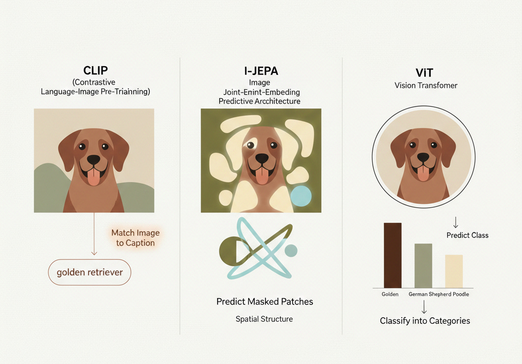
I-JEPA (Image Joint-Embedding Predictive Architecture) is Meta’s self-supervised vision model. The core idea is elegantly simple: take an image, mask out large regions, and train the model to predict the representations of those masked regions using only the visible context.
But here’s the critical design choice—I-JEPA predicts in latent space, not pixel space. Unlike a masked autoencoder (MAE) that reconstructs raw pixels, I-JEPA predicts the abstract representation of what’s missing. This forces the model to learn high-level semantic structure rather than low-level texture details.
The architecture uses a context encoder ( f_theta ) and a target encoder ( f_theta bar) (an exponential moving average of the context encoder). Given an image ( x ), a context block ( B_c ), and target blocks ( B_t^1, ..., B_t^M ):
where ( sg ) is the stop-gradient operator. The predictor is a lightweight transformer that takes the context encoder’s output and predicts the target representations at specific spatial positions.
What makes this interesting for our experiment: I-JEPA embeddings should encode spatial structure and part-whole relationships the kind of understanding you’d want for reasoning about where things are, not just what they are.
Model used: facebook/ijepa_vith14_1k (ViT-Huge/14, 632M params, trained on ImageNet)
CLIP: Language-Aligned Vision
CLIP (Contrastive Language-Image Pre-training) takes a fundamentally different approach. It trains a vision encoder and a text encoder jointly on 400 million image-text pairs from the internet, using a contrastive objective:
where ( v_i ) and ( t_i ) are the vision and text embeddings for the (i)-th pair, ( sim ) is cosine similarity, and ( tau ) is a learned temperature parameter.
The result: CLIP’s vision embeddings are already aligned with language. When CLIP looks at a golden retriever, its embedding is close to the text embedding of “golden retriever” in the shared space. This is a massive head start when you’re trying to bridge vision into a language model.
Model used: openai/clip-vit-large-patch14 (ViT-Large/14, 304M params, contrastive pre-training on 400M pairs)
ViT: The Supervised Baseline
The standard Vision Transformer, trained with old-school supervised classification on ImageNet-21k. No fancy self-supervised objectives, no language alignment. Just “here’s an image, predict the class.”
The ViT embedding space is organized around class-discriminative features. It knows that golden retrievers look different from German shepherds, but it has no concept of “golden” as a word or “retriever” as a role. It’s purely visual.
Model used: google/vit-large-patch16-224 (ViT-Large/16, 304M params, supervised on ImageNet-21k)
How Do These Embeddings Actually Differ?
All three models take an image and produce a sequence of patch tokens—one embedding vector per image patch. But the information encoded in those vectors is radically different:
Same image, three completely different internal representations. The question is: which representation gives a language model the best foundation for visual understanding?
Model Stitching: Turning an LLM into a VLM
The General Idea
A Vision-Language Model (VLM) is, at its core, a language model that can also see. The simplest way to build one: take a pre-trained vision encoder, take a pre-trained LLM, and learn a mapping between their embedding spaces.
This is sometimes called “model stitching” or “LLM-centric VLM training.” The idea has been popularized by models like LLaVA, which showed that you can get surprisingly good multimodal performance by just training a linear projection layer between a frozen CLIP encoder and a frozen LLM.
How Does It Work?
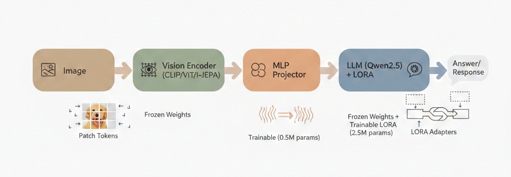
The pipeline looks like this:
Image → Patch Tokens: The vision encoder processes the image and outputs a sequence of patch embeddings. For a ViT-Large/14, a 224×224 image becomes 256 patch tokens, each a 1024-dimensional vector.
Projection: A small trainable MLP maps the vision embeddings from the encoder’s dimension to the LLM’s embedding dimension:
where ( z_vision in R^{N x d_v} ) are the patch tokens and ( h_visual is an element of R^(N x d_llm) ) are the projected visual tokens.
Concatenation: The projected visual tokens are prepended to the text token embeddings:
LLM Forward Pass: The combined sequence is fed into the LLM, which processes it with its standard transformer layers. The LLM doesn’t “know” the first N tokens came from an image, it just sees a sequence of embeddings.
Loss: Computed only on the text response portion (the answer), not on the visual tokens or the instruction/question tokens.
Ways to Do This
There are a few variants of this approach:
Frozen encoder + Frozen LLM + Linear projection (simplest): Just train a single linear layer. This is what LLaVA-v1 did initially.
Frozen encoder + Frozen LLM + MLP projection (what we do): A 2-layer MLP gives the projection more capacity to handle non-trivial embedding space misalignment.
Frozen encoder + LoRA on LLM + MLP projection (what we do): Adding LoRA adapters to the LLM’s attention layers lets it learn to attend to visual tokens differently, without modifying the base weights. This is parameter-efficient and gives a nice bump in quality.
Full fine-tuning: Unfreeze everything. Expensive, risks catastrophic forgetting, and doesn’t let you isolate the encoder’s contribution—which is what we care about here.
Our Methodology
The Setup
The goal is to isolate the effect of the vision encoder. So we hold everything else constant:
For each of the three vision encoders, we:
Freeze the vision encoder completely no gradients flow back.
Freeze the LLM base weights.
Train only the projector MLP (~0.5M params) and LoRA adapters on
q_projandv_proj(~2.5M params).Measure training loss convergence and downstream VQA accuracy.
The total trainable parameters are roughly 3M per run—about 0.3% of the full model. Everything else is frozen.
Projector Architecture
The projector is a simple 2-layer MLP with layer normalization:
LayerNorm(d_vision) → Linear(d_vision, d_llm) → GELU → Linear(d_llm, d_llm)For CLIP and ViT (1024-dim) mapping to Qwen2.5-0.5B (896-dim), this is a 1024 → 896 → 896 MLP. For I-JEPA (1280-dim), it’s 1280 → 896 → 896.
LoRA Configuration
We apply LoRA (Low-Rank Adaptation) to the LLM’s attention layers:
where ( B is an element of R^(d x r) ), ( A is an element of R^(r x d) ), ( r = 16 ), and ( alpha = 32 ). Applied to q_proj and v_proj in every attention layer.
Two Experiments
We ran two experiments with different LLM scales and datasets:
Experiment 1 — 0.5B + COCO-QA
Experiment 2 — 1.5B + VQAv2
Results
Experiment 1: 0.5B LLM + COCO-QA
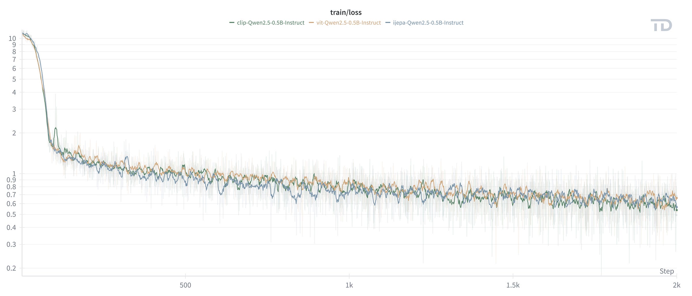
Training Loss:
Something immediately interesting: I-JEPA reaches the lowest final loss (0.49) despite having fewer trainable parameters as a percentage. ViT is second (0.52), and CLIP is actually highest (0.68). But don’t jump to conclusions from training loss alone—what matters is how well these models generalize.
Evaluation Accuracy (exact match, 1K samples per benchmark):
Now it gets interesting. CLIP dominates on COCO-QA (55.8%) not surprising, since COCO-QA is basically “name the thing in the image” and CLIP’s embeddings are literally optimized for object-level language alignment. But on CLEVR (compositional reasoning ”how many red cubes are left of the blue sphere?”), I-JEPA and ViT both outperform CLIP by 2x.
All three completely fail at TallyQA (counting). With a 0.5B LLM and 2,000 training steps, none of them can count.
Experiment 2: 1.5B LLM + VQAv2
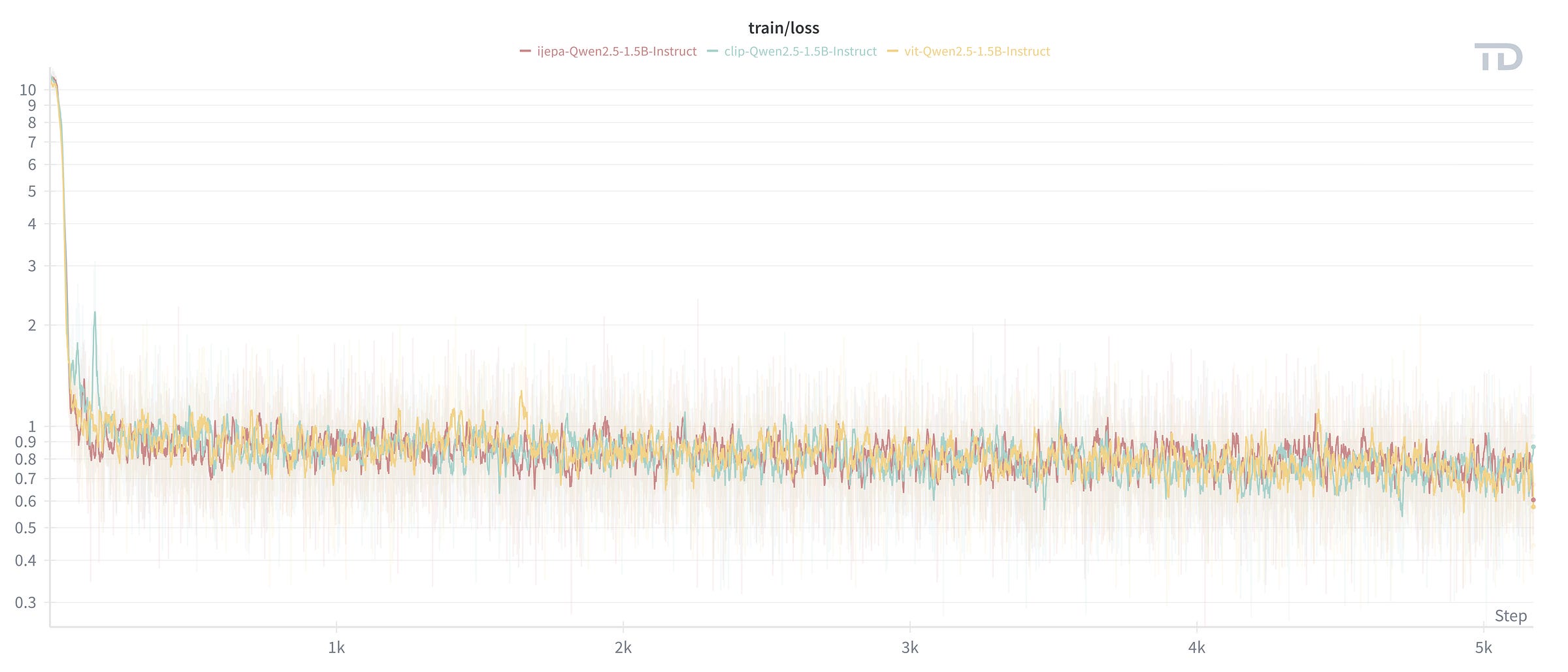
Training Loss:
All three reach similar avg_last50 losses (~0.73-0.75), despite different final loss values. CLIP shows the lowest minimum loss (0.25) but the highest final loss (0.93)—it’s more spiky. VIT is the most stable.
Evaluation Accuracy (exact match, 1K samples per benchmark):
With the 1.5B LLM, everything changes. CLIP goes from 20.3% to 37.5% average—a massive jump. CLIP and I-JEPA are tied on CLEVR (35.4%), which is remarkable: I-JEPA’s self-supervised structural understanding matches CLIP’s language-aligned representations on compositional reasoning tasks. And all three can now actually count (TallyQA: 38-44%)—the extra LLM capacity made the difference.
The 0.5B vs 1.5B Story
CLIP benefits the most from scaling. This makes intuitive sense: CLIP embeddings are already language-aligned, so a more capable LLM can extract more from them. The projection bottleneck matters less when the LLM has more capacity to “understand” the projected visual tokens.
I-JEPA’s improvement is more modest, but its CLEVR score tells a different story—it matches CLIP on spatial reasoning. I-JEPA’s structural understanding might become even more valuable for tasks where spatial reasoning matters more than object naming.
What I Learned
1. CLIP’s language alignment is a genuine unfair advantage for VLMs. When your vision embeddings already live near the right words, the projector’s job becomes trivially easy. This is why CLIP is the default choice for VLM builders, and after running this experiment, I get it.
2. I-JEPA is the underdog to watch. It matches CLIP on compositional reasoning (CLEVR) despite having zero text supervision during pre-training. For tasks that care about structure—spatial reasoning, counting, scene understanding I-JEPA’s representation might actually be superior. The fact that it achieves 35.4% on CLEVR with pure self-supervised pre-training is genuinely impressive.
3. The LLM scale matters more than the encoder (to a point). Going from 0.5B to 1.5B gave a bigger accuracy boost than any encoder swap. This suggests that, beyond a baseline quality threshold, the LLM’s ability to reason about visual tokens matters more than the raw quality of those tokens.
4. Model stitching is surprisingly effective. With only ~3M trainable parameters (0.3% of the total model), we get functional VQA performance. The projector + LoRA combination, it gives the LLM just enough flexibility to bridge the modality gap without destroying its language capabilities.
Future Improvements
There’s a lot of low-hanging fruit here:
Higher LoRA rank (32-64): The 1.5B model might be under-adapted with rank 16. More LoRA parameters could help, especially for I-JEPA where the embedding space is more “alien” to the LLM.
More LoRA targets: Currently only adapting
q_projandv_proj. Addingk_proj,o_proj,gate_proj,up_proj,down_projwould give the LLM more room to restructure its attention patterns for visual inputs.Multi-epoch training: We only ran 1 epoch on VQAv2. The loss curves still have room to improve—2-3 epochs would likely help.
Larger LLMs (3B, 7B): The 0.5B → 1.5B scaling curve suggests diminishing returns haven’t kicked in yet. A 7B LLM with the same setup could be dramatically better.
Multi-dataset training: Training on a mix of VQAv2, COCO-QA, ScienceQA, and visual dialogue datasets would improve generalization.
V-JEPA as encoder: The video-native V-JEPA model, using individual frame embeddings, could provide even richer spatiotemporal representations. This is the experiment I originally wanted to run.
Softer evaluation metrics: Exact match is harsh. Token-level F1, BERTScore, or human evaluation would give a more nuanced picture of model quality.
Conclusion
I set out to answer a simple question: does the vision encoder’s pre-training strategy matter for VLM stitching? The answer is yes—but it’s nuanced.
CLIP wins on average, and it wins convincingly when paired with a larger LLM. Its language-aligned embeddings give the projector an easy job and the LLM a familiar representation to work with. If you’re building a VLM and want maximum performance with minimal fuss, CLIP is still the right default.
But I-JEPA is the more interesting story. It matches CLIP on compositional reasoning tasks despite never seeing a single word during pre-training. Its self-supervised structural understanding captures something that contrastive text alignment doesn’t—spatial relationships, part-whole hierarchies, scene geometry. As vision tasks move beyond “name the object” toward genuine spatial reasoning, I-JEPA-style representations might become increasingly valuable.
And the supervised ViT baseline deserves more respect. It consistently sits between CLIP and I-JEPA, proving that good old ImageNet-supervised features are still competitive as a starting point for VLMs.
The code, trained weights, and evaluation scripts are all open:
Trained Models (0.5B): huggingface.co/Teen-Different/CLIP-ViT-IJEPA-VLMs-0.5B
Trained Models (1.5B): huggingface.co/Teen-Different/CLIP-ViT-IJEPA-VLMs-1.5B
If you want to reproduce the results or try stitching a different encoder, the whole setup is designed to make that easy—swap the model ID in the config, run train.py done.
References
I-JEPA — Assran, M., et al. “Self-Supervised Learning from Images with a Joint-Embedding Predictive Architecture.” CVPR 2023. arXiv:2301.08243
V-JEPA — Bardes, A., et al. “V-JEPA: Latent Video Prediction for Visual Representation Learning.” Meta AI, 2024. arXiv:2404.16930
CLIP — Radford, A., et al. “Learning Transferable Visual Models From Natural Language Supervision.” ICML 2021. arXiv:2103.00020
ViT — Dosovitskiy, A., et al. “An Image is Worth 16x16 Words: Transformers for Image Recognition at Scale.” ICLR 2021. arXiv:2010.11929
LLaVA — Liu, H., et al. “Visual Instruction Tuning.” NeurIPS 2023. arXiv:2304.08485
LoRA — Hu, E., et al. “LoRA: Low-Rank Adaptation of Large Language Models.” ICLR 2022. arXiv:2106.09685
Qwen2.5 — Qwen Team. “Qwen2.5 Technical Report.” 2024. qwen2.5
The Cauldron — HuggingFace M4 Team. “The Cauldron: A Multimodal Dataset Collection.” huggingface.co/datasets/HuggingFaceM4/the_cauldron


