Sample-Tuned Rank-Augmented Weights

An experiment in making neural networks rewrite themselves for every single input. Inspired by the human brain.

The way we currently do deep learning is kind of weird. We train these massive, models Transformers, CNNs, whatever and once training is done, they are frozen. They are static statues.

When you run inference, the weights are exactly the same whether the input is a picture of a cat, a complex math proof, or a blurry photo of a receipt. The model forces the data to fit its rigid structure.

But that’s not how biology works. Your brain isn’t a static graph. If you are solving a math problem, your brain doesn’t just “activate” neurons, it chemically modulates synaptic efficiency on the fly. It adapts the processing machinery to the input.

This article introduces STRAW (Sample-Tuned Rank-Augmented Weights). It’s a simple but slightly crazy experiment to see if we can make a model that shape-shifts its own weights for every single input sample.

We aren’t fitting data to the model anymore; we are fitting the model to the data.

Inspiration

My initial hypothesis didn’t actually start with weight generation. It started with a question: Why are our networks static during Supervised Fine-Tuning (SFT)?

I originally imagined an architecture involving a secondary Reinforcement Learning (RL) agent that would “watch” the main model during SFT. The idea was to have this RL agent dynamically expand or contract the network topology in real-time.

\(\text{Action}_{RL} \in \{ \text{Add Neuron}, \text{Delete Neuron} \}\)

If the loss was high, the agent would inject new neurons. If the loss was low, it would prune connections. The goal was a living network that physically adapted its size to the difficulty of the problem.

But there was a massive roadblock: Differentiability. You can’t easily backpropagate through discrete structural changes like “deleting a node” while simultaneously training weights via SGD. The gradients break, and the training loop becomes a nightmare of instability.

So, I pivoted. I realized I didn’t need to change the structure (the graph); I just needed to change the flow.

This led me to neuromodulation, which is how biology solves this exact problem without needing to grow new physical neurons every millisecond.

In the brain, you have your standard electrical signals (action potentials), but you also have a “soup” of chemicals (dopamine, serotonin, acetylcholine) that float around and change how likely neurons are to fire. They effectively change the “weights” of the network dynamically based on context and internal state.

Current neural networks connect every neuron to every neuron with a fixed scalar weight w. STRAW asks: What if w wasn’t a number, but a function of the input?

\(w = f(input, context)\)

This creates what I call an “Infinite Expert” system. The model isn’t one generalist trying to cover the distribution of all data. It is a generator that creates a specific, temporary “expert” model for the exact millisecond it sees a specific image, processes it, and then dissolves.

Background

You might be thinking, “Isn’t this just a HyperNetwork?”

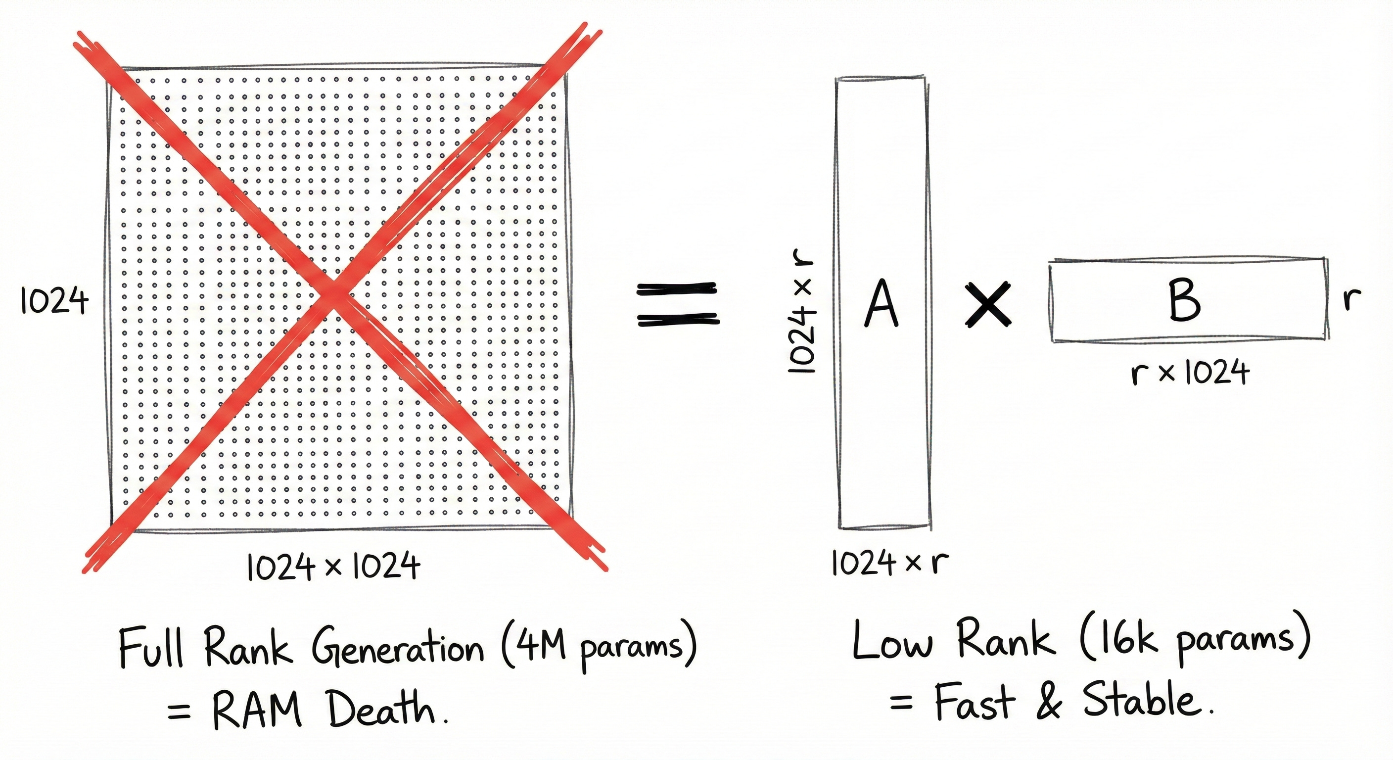
HyperNetworks (Ha et al.) generate weights for another network. But generating a full weight matrix is computationally suicidal.

For a layer mapping dimension d_in to d_out:

\( N_{params} = d_{in} \times d_{out} \)

If you have a layer with dimensions 2048 * 2048, that’s roughly 4 million parameters. To generate that per sample, your generator needs to output 4 million numbers. That explodes memory and is impossible to train stably.

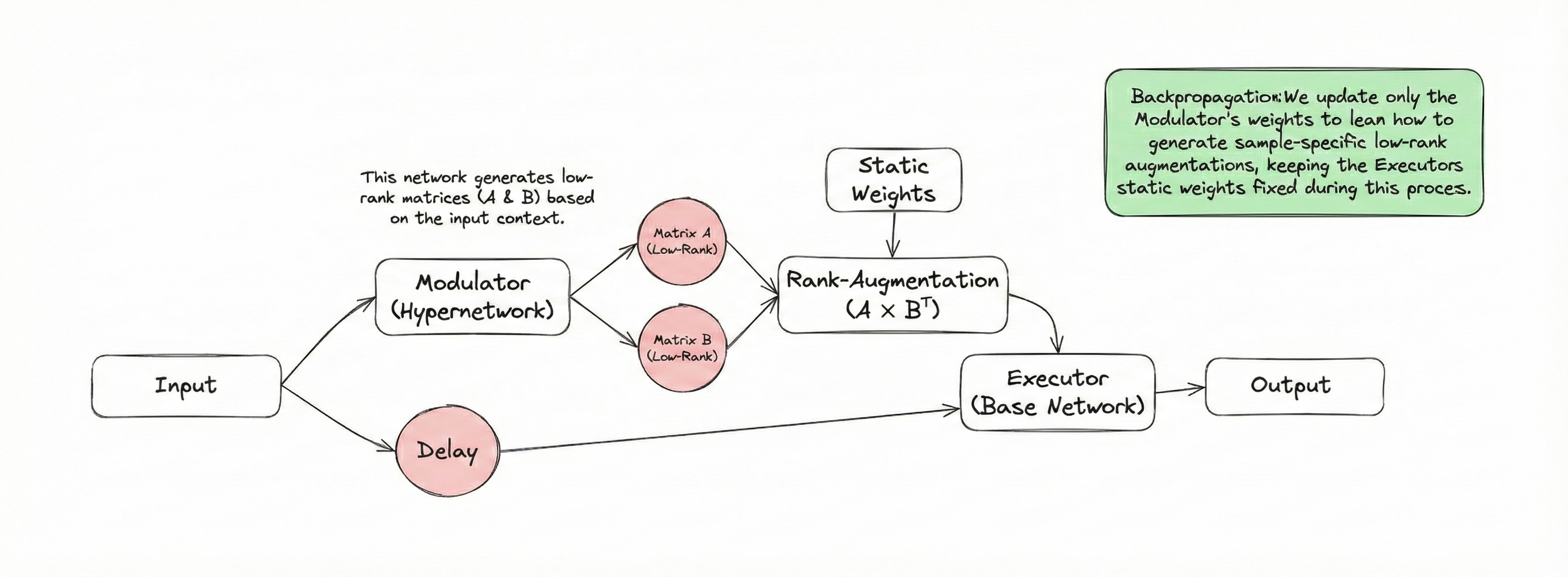
Methodology

Our architecture separates the neural mechanism into two distinct agents:

1. The Modulator: A HyperNetwork that observes the input context.

2. The Executor: The base network that performs the task.

The Low-Rank Decomposition

Instead of generating the full Delta_W, we assume that the necessary adaptation for any given sample lies in a low-dimensional subspace. We use the LoRA (Low-Rank Adaptation) formulation, but make it dynamic.

We decompose the weight update into two low-rank matrices, A and B:

\(\Delta W(x) = A(x) \cdot B(x)^\top\)

Where the rank r is a hyperparameter such that:

\(r \ll \min(d_{in}, d_{out})\)

The Pipeline

The forward pass for a single sample x proceeds in three steps.

Step 1: Context Encoding

The Modulator scans the input x to produce a latent “style” vector z. This vector encapsulates the “vibe” or context of the input (e.g., “this image is rotated” or “this is a blurry font”).

Failed to render LaTeX expression — no expression found

\(z = \text{Encoder}(x), \quad z \in \mathbb{R}^{d_{latent}}\)

Step 2: Weight Generation

A projection network Phi maps this latent vector to a flat vector of parameters, which are then reshaped into our rank decomposition matrices.

\(\theta = \Phi(z)\)

\(\theta \rightarrow \{ A(x), B(x) \}\)

Here, the dimensions are highly efficient:

\(A(x) \in \mathbb{R}^{d_{out} \times r}\)

\(B(x) \in \mathbb{R}^{d_{in} \times r}\)

Step 3: The Adaptive Forward Pass

The Executor computes the final output using the base weights augmented by the generated weights.

\(y = (W_{static} + \alpha (A(x) B(x)^\top)) x + b\)

This operation is computationally cheap because we never actually materialize the full d_out * d_in matrix. We use the associative property of matrix multiplication:

\((A B^\top) x = A (B^\top x)\)

This reduces the complexity from quadratic O(d^2) to linear-rank O(dr).

Complexity Analysis

Let’s look at the parameter savings. For a standard weight matrix W:

\(\text{Cost}_{standard} = d_{in} \cdot d_{out}\)

For STRAW, the generator only predicts:

\(\text{Cost}_{STRAW} = (d_{in} + d_{out}) \cdot r\)

If d=1024 and r=8:

\(\frac{d^2}{2dr} = \frac{1048576}{16384} \approx 64\text{x reduction}\)

This 64x reduction is the only reason this approach is trainable on consumer hardware.

Experiments

We wanted to test if this added complexity actually helps the model generalize, or if it’s just fancy math for no reason.

Setup

• Dataset: EMNIST (Balanced). It’s like MNIST but harder (letters and numbers).

• Test Variations:

  1. Standard: Just the clean images.

  2. Rotated: Random rotations 60 degrees to test spatial robustness.

  3. Blurred: Gaussian blur to test feature degradation.

• Data Scarcity: We trained on 100%, 20%, and 10% of the data to see if STRAW helps when data is low (few-shot capabilities).

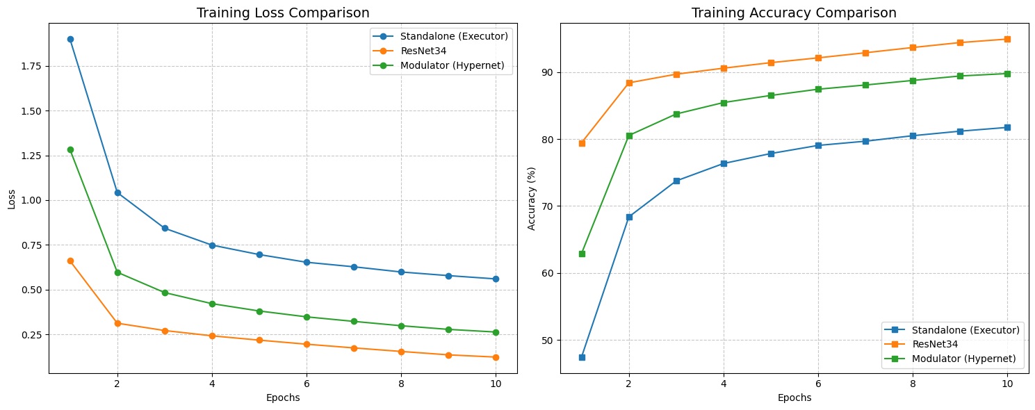
Contenders

1. Standalone (Baseline): A standard CNN Executor.

2. ResNet34 (Industry Standard): A slightly modified ResNet to fit the image size.

3. STRAW (Modulator): Our dynamic rank-16 hyper-model.

Results

Let’s look at the numbers. We aren’t trying to claim State-of-the-Art (SOTA) here—we are trying to prove that a neural network can successfully modify its own weights in real-time without collapsing into noise. To test this, we ran three distinct experimental sets, keeping the test set constant across all runs to ensure fair comparisons.

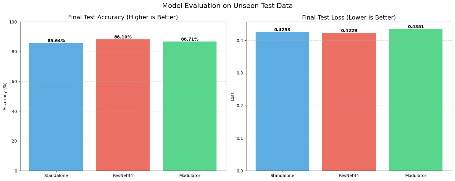
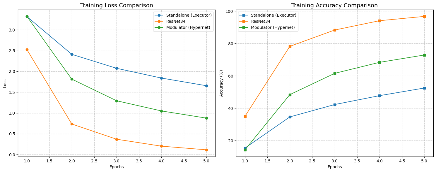
Set 1: The Full Dataset Baseline

First, we trained on the complete, balanced EMNIST dataset. As expected, the industry-standard ResNet34 was the king of the hill, achieving a test accuracy of roughly 88.10% with a loss of 0.4229. It’s a deep, residual architecture designed exactly for this kind of work, so that’s no surprise.

The real comparison, however, is between our STRAW (Modulator) and the Standalone baseline. The Standalone model managed 85.64% accuracy. STRAW, running with a rank of 16, outperformed it, hitting 86.71%. While a 1% gain might look small, it proves the fundamental hypothesis: the Modulator isn’t just adding noise. It is successfully “guessing” a better weight configuration for each specific image than the static model could achieve on its own.

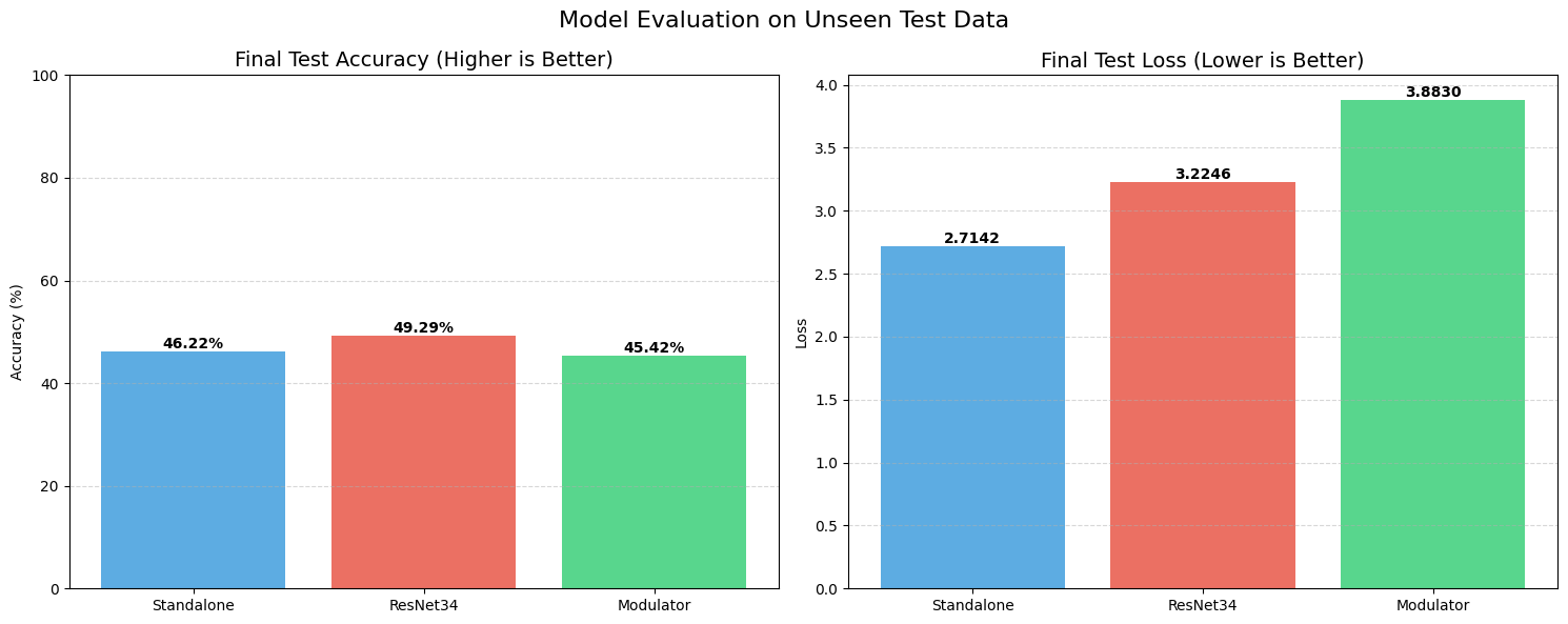
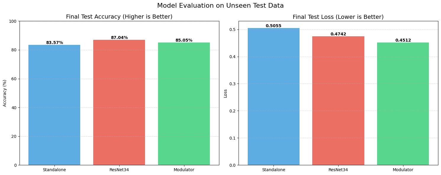
We also threw curveballs at the models. On the Rotated test set, all models struggled, dropping to the 45-49% range. This indicates that our current Modulator isn’t yet smart enough to intuitively understand “rotation” as a geometric concept. However, on the Blurred dataset, STRAW maintained a solid 85.05% accuracy, showing it can adapt to feature degradation better than the Standalone model, which dropped lower.

Performance on standard test data

Performance on rotated test data

Performance on blurred test data

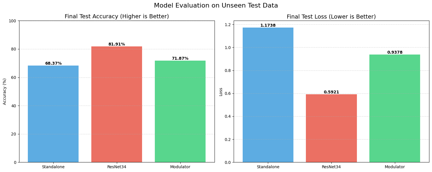
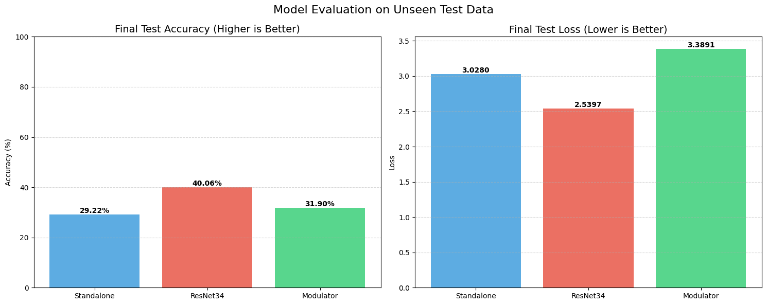
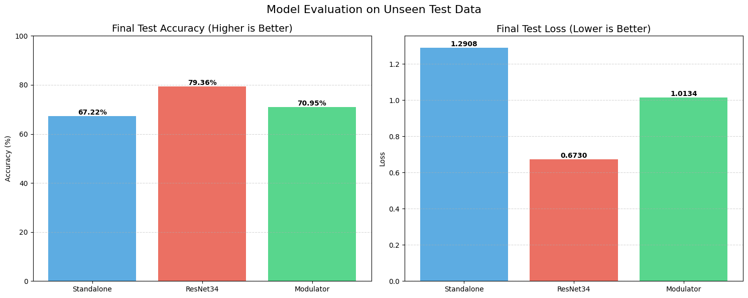
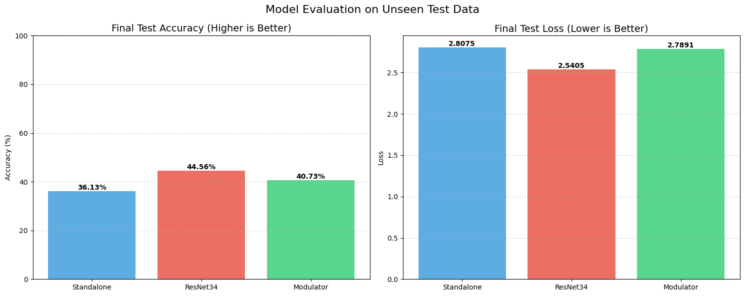
Set 2: The “Starvation” Test (10% Data)

Things got much more interesting when we starved the models of data. We trained on only 10% of the dataset to see which architectures would collapse.

The Standalone model struggled significantly here. It couldn’t generalize well, hitting a test accuracy of only 68.37% with a massive loss of over 1.1. It essentially started memorizing and guessing.

STRAW, however, acted as a regularizer. Even with this tiny amount of training data, the Modulator managed to push the test accuracy up to 71.87%, with a lower loss of 0.93. It shows that when data is scarce, having a dynamic weight generator helps the model adapt to unseen examples better than a static set of weights can.

Performance on standard test data

Performance on rotated test data

Performance on blurred test data

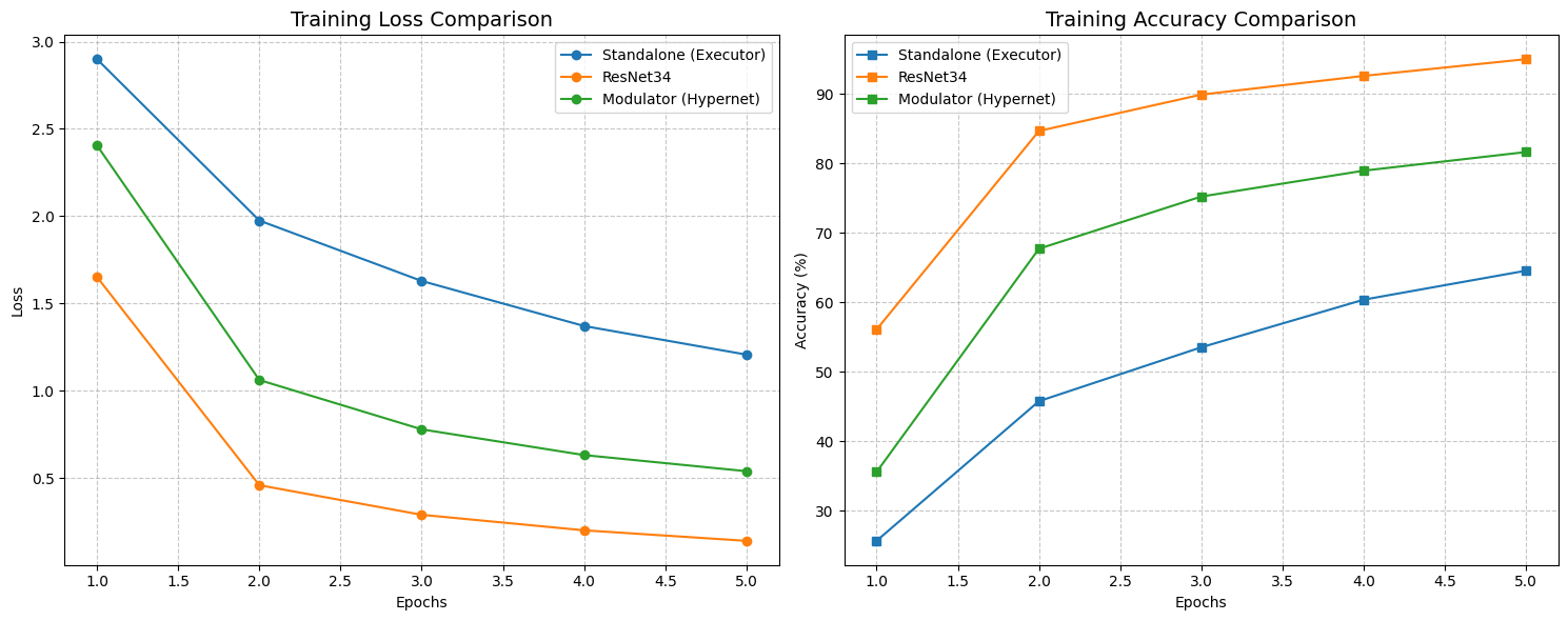
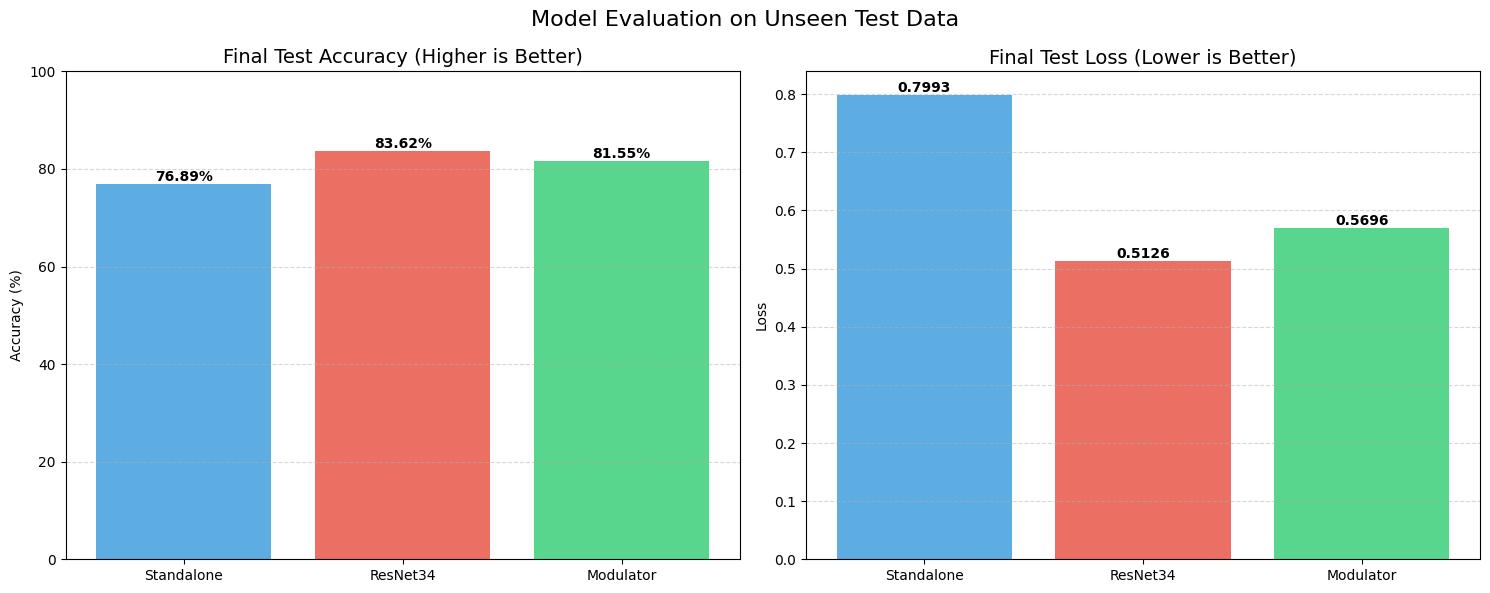
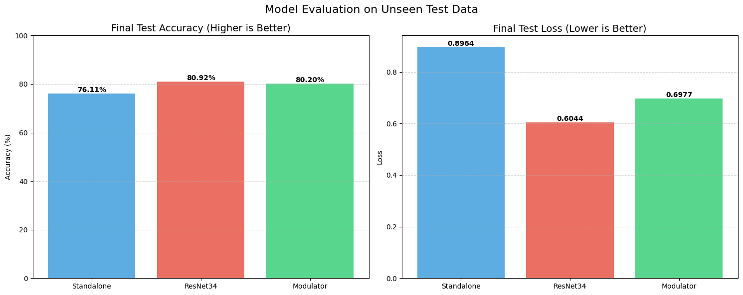
Set 3: Scaling Up (20% Data, Rank 32)

For the final set, we doubled the data to 20% and, crucially, doubled the capacity of our approach by increasing the rank from 16 to 32.

The gap between our experimental approach and the industry standard narrowed significantly. The Standalone model hit 76.89%. ResNet34 sat at 83.62%. But STRAW (Rank 32) climbed to 81.55%.

We are now within 2% of a heavy, optimized ResNet, using a weird, experimental architecture that rewrites its own brain on the fly. This suggests that the “capacity” of our adaptation is directly tied to the rank—meaning if we scale this up further, we might actually catch or surpass the residual baselines.

Performance on standard test data

Performance on rotated test data

Performance on blurred test data

Discussion…It’s Alive

So, what does this tell us? Let’s be real: did we beat the State-of-the-Art? Sadly, no. ResNet34 is still the deeper, more stable beast for pure image classification.

But the failure to beat SOTA is largely due to our Modulator network (The Eye). Currently, it’s a simple CNN. It looks at a rotated “7” and just sees weird pixels; it doesn’t intuitively understand “Oh, this is a 7 that has been turned 60 degrees.” Because the Eye is weak, the instructions it sends to the Executor are imperfect.

However, the fact that this works at all is the breakthrough. In HyperNetwork research, generating weights usually leads to exploding gradients or total mode collapse. STRAW stabilized. It learned to map inputs to specific weight configurations that are measurably better than static weights. The Rank 32 experiment proves that this isn’t a fluke—it’s a scalable property. We essentially built a model that functions like a biological circuit, modulating its own synapses based on input flow, and it actually learned to see.

Conclusion

STRAW is a step toward “Liquid Neural Networks.” By utilizing low-rank decomposition, we bypassed the curse of dimensionality that usually kills HyperNetworks.

We showed that a model can effectively rewrite its own wiring for every single image it sees. While we didn’t beat the heavily optimized ResNet34 (yet), the fact that a self-modifying network stabilized and performed within striking distance of a standard architecture on limited data is a massive win.

It demonstrates that deep learning models don’t have to be static statues. They can be fluid, adaptive systems.

The real endgame here is figuring out how to properly “drive” the Modulator. It’s not just about feeding it pixels, it’s about making it smart enough to actually understand the geometry so if it sees a rotated or skewed image, it intuitively knows to generate “rotated weights” to compensate. I’ve got a specific, slightly wild concept in mind for the next experiment to force this separation between “seeing” and “understanding,” potentially using context that goes way beyond just the image itself. I won’t spill the details yet (mostly because it might completely crash and burn), but if we can crack that level of dynamic adaptation, we are going to witness something entirely new.

It’s not AGI, but it’s definitely not static.

Code’s up on GitHub if you want to dig in: https://github.com/REDDITARUN/STRAW

If you want to follow along past this blog: https://bento.me/tarunreddi

References

• Ha, D., Dai, A., & Le, Q. V. (2016). HyperNetworks. arXiv preprint arXiv:1609.09106.

• Hu, E. J., Shen, Y., Wallis, P., Allen-Zhu, Z., Li, Y., Wang, S., Wang, L., & Chen, W. (2021). LoRA: Low-Rank Adaptation of Large Language Models. arXiv preprint arXiv:2106.09685.

• Mastrogiuseppe, F., & Ostojic, S. (2018). Linking Connectivity, Dynamics, and Computations in Low-Rank Recurrent Neural Networks. Neuron, 99(3), 609-623. (Note: The title in your draft was slightly different (”Chaos” instead of “Computations”), but this is the correct citation for the Mastrogiuseppe & Ostojic paper regarding low-rank connectivity).

• Perez, E., Strub, F., de Vries, H., Dumoulin, V., & Courville, A. (2018). FiLM: Visual Reasoning with a General Conditioning Layer. AAAI Conference on Artificial Intelligence.